


Coming soon
The FieldKit Blog
Born in the Field
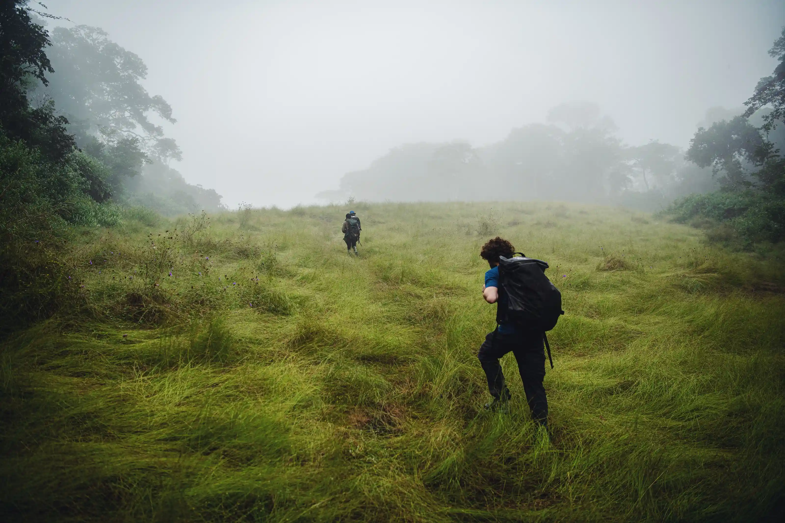
Flashback to 2016: our founder, Shah Selbe, was working alongside National Geographic’s Okavango Wilderness Project to document and protect one of Africa’s most pristine wetland ecosystems. To support the team’s scientific goals, we cobbled together a DIY sensor network from open hardware, streaming live data on pH, temperature, and water flow from one of the world’s most remote river systems. It was early proof that transparent, low-cost tech could connect distant ecosystems and support urgent conservation efforts. Thus began our dream of building the “Internet of Earth Things” — a resilient network of environmental sensors that could empower real-time, open-source conservation science.